Generative Deep Learning
What is Generative Modeling?
Generative modeling is a branch of machine learning that involves training a model to produce new data that is similar to a given dataset
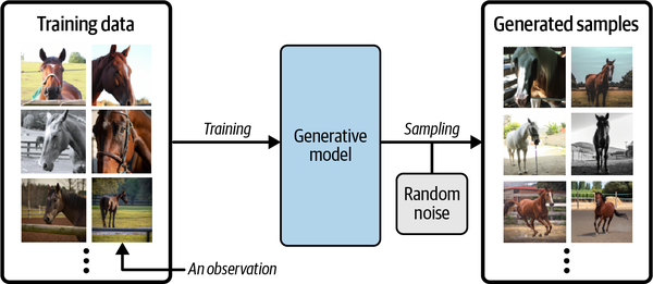
We can sample from this model to create novel, realistic images of horses that did not exist in the original dataset.
One data point in the training data is called as observation. Each observation consists of many features.
A generative model must be probabilistic rather than deterministic, because we want to be able to sample many different variations of the output, rather than get the same output every time.
Generative Versus Descriminative Modeling
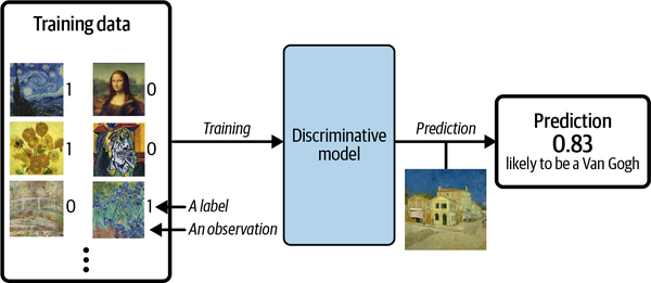
Figure 1-2 shows the discriminative modeling process.
Generative modeling doesn’t require the dataset to be labeled because it concerns itself with generating entirely new images, rather than trying to predict a label of a given image.
Conditional Generative Models
For example, if out dataset contains different types of fruit, we could tell our generative model to specifically generate an image of an apple.
The Rise of Generative Modeling
Until recently, discriminative modeling has been the driving force behind most progress in machine learning. This is because the corresponding generative modeling problem is typically much more difficult to tackle.
However, as machine learning technologies have matured, this assumption has gradually weakened.
In the last 10 years many of the most interesting advancements in the field have come through novel applications of machine learning to generative modeling tasks.
Generative services that target specific business problems
- generate original blog posts given a particular subject matter
- produce a variety of images of your product in any setting
- write social media content and ad copy to match your brand
- game design and cinematography to output video and music
Generative Modeling and AI
There are three deeper reasons why generative modeling can be considered the key to unlocking a far more sophisticated form of artificial intelligence that goes beyond what discriminative modeling alone can achieve.
Firstly, we shouldn’t limit our machine training to simply categorizing data and should also be concerned with training models that capture a more complete understanding of the data distribution. Many of the same techniques that have driven development in discriminative modeling, such as deep learning, can be utilized by generative models too.
Secondly, generative modeling is now being used to drive progress in other fields of AI, such as reinforcement learning. A traditional approach(to train a robot to walk across a terrain) is fairly inflexible because it is trained to optimize the policy for one particular task. An alternative approach that has recently gained traction is to train the agent to learn a world model (not the real environment)of the environment using a generative model, independent of any particular task.
Finally, if we are to say that we have built a machine that has acquired a form of intelligence, generative modeling must surely be part of the solution. Current neuroscientific theory suggests that our perception of reality is not a highly complex discriminative model operating on our sensory input to produce predictions of what we are experiencing, but is instead a generative model that is trained from birth to produce simulations of our surroundings that accurately match the future.
The Generative Modeling Framework
- We have a dataset of observation X.
- We assume that the observations have been generated according to some unknown distribution, Pdata
- We want to build generative model Pmodel that minics Pdata. If we achieve this goal, we can sample from Pmodel to generate observations that appear to have been drawn from Pdata.
- Therefore, the desirable properties of Pmodel are:
- Accuracy
If Pmodel is high for a generated observation, it should look like it has been drawn from Pdata. if Pmodel is low for a generated observation, it should not look like it has been drawn from Pdata.- Generation
It should be possible to easily sample a new observation from Pmodel.- Representation
It should be possible to understand how different high-level features in the data are represented by Pmodel.
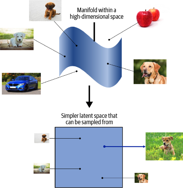
Representation Learning
Instead of trying to model the high-dimensional sample space directly, we describe each observation in the training set using some lower dimensional latent space and then learn a mapping function that can take a point in the latent space and map it to a point in the original domain. In other words, each point in the latent space is a representation of some high-dimensional observation.
One of the benefits of training models that utilize a latent space is that we can perform operations that affect high-level properties of the image by manipulating its representation vector within the more manageable latent space.
The concept of encoding the training dataset into a latent space so that we can sample from it and decode the point back to the original domain is common to many generative modeling technique.
Core Probability Theory
Five key terms
Sample space
- The sample space is the complete set of all values an observation x can take
Probability density function (or simply density function)
- a function p(x) that maps a point x in the sample space to a number between 0, and 1. The integral of the density function over all points in the sample space must equal 1, so that it is a well-defined probability distribution.
Parametric modeling
- a technique that we can use to structure our approach to finding a suitable Pmodel(x)
Likelihood
- The likelihood ℒ(θ|𝐱) of a parameter set θ is a function that measures the plausibility of θ , given some observed point 𝐱
Maximum likelihood estimation
Generative Model Taxonomy
While all types of generative models ultimately aim to solve the same task, they all take slightly different approaches to modeling the density function. There are three possible approaches:
- Explicitly model the density function, but constrain the model in some way, so that the density function is tractable(i.e., it can be calculated).
- Explicitly model a tractable approximation of the density function.
- Implicitly model the density function, through a stochastic process that directly generates data.
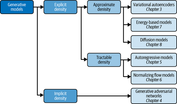
The best-known example of an implicit generative model is a generative adversarial network.
Approximate density models include variational autoencoders.
A common thread that runs through all of the generative model family types is deep learning
Deep Learning
Deep Neural Networks
The majority of deep learning systems are artificial neural networks(ANNs, or just neural networks for short) with multiple stacked hidden layers.
What is a Neural Network?
A neural network consists of a series of stacked layers. Each layer contains units that are connected to the previous layer’s units through a set of weights.
One of the most common layers is the fully connected (or dense) layer that connects all units in the layer directly to every unit in the previous layer.
Neural networks where all adjacent layers are fully connected are called multilayer perceptrons(MLPs).
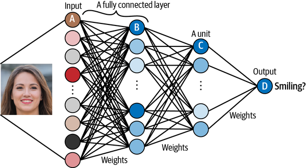
Let’s walk through the network shown in figure 2-2
- Unit A receives the value for an individual channel of an input pixel
- Unit B combines its input values so that it fires strongest when a particular low-level feature such as an edge is present.
- Unit C combines the low-level features so that it fires strongest when a higher-level feature such as teeth are seen in the image.
- Unit D combines the high-level features to that it fires strongest when the person in the original image is smiling.
The layers between the input and output layers are called hidden layers.
Multilayer Perceptron(MLP)
The MLP is a discriminative (rather than generative) model, but supervised learning will still play a role in many types of generative models.
Preparing the Data -> Building the Model(Layers, Activation functions) -> Compiling the Model(Loss functions, Optimizers) -> Training the Model -> Evaluating the Model
- There are many kinds of activation function, but three of the most important are ReLU(rectified linear unit), sigmoid, and softmax.
- Three of the most commonly used loss functions are mean square error, categorical cross-entropy, and binary cross entropy.
- One of the most commonly used and stable optimizer is Adam(Adaptive Moment Estimation).
Convolutional Neural Network(CNN)
To make the network perform well, the spatial structure of the input images needs to be taken into account.
Convolutional Layers
The convolution is performed by multiplying the filter pixel-wise with the portion of the image, and summing the results. The output is more positive when the portion of the image closely matches the filter and more negative when the portion of the image is the inverse of the filter.
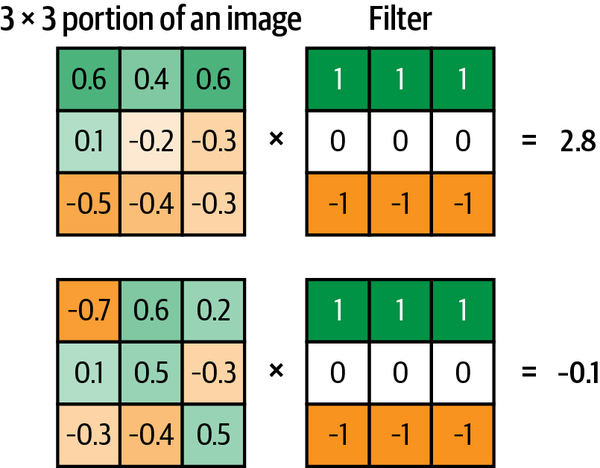
If we move the filter across the entire image from left to right and top to bottom, recording the convolutional output as we go, we obtain a new array that picks out a particular feature of the input, depending on the values in the filter.
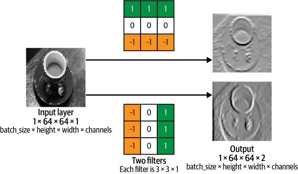
A convolutional layer is simply a collection of filters, where the values stored in the filters are the weights that are learned by the neural network through training. Initially these are random, but gradually the filters adapt their weights to start picking out interesting features such as edges or particular color combinations.
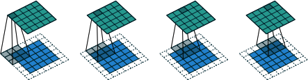
padding = "same" and strides = 1, to generate the 5 x 5 x 1 output (green)Stride
The strides parameter is the stop size used by the layer to move the filters across the input. Increasing the stride therefore reduces the size of the output tensor.
Padding
The padding = "same" input parameter pads the input data with zeros so that the output size from the layer is exactly the same as the input size when strides = 1.
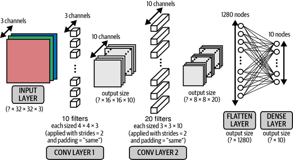
Stacking convolutional layers
The output of a Conv2D layer is another four-dimensional tensor, now of shape (batch_size, height, width, filters), so we can stack Conv2D layers on top of each other to grow the depth of our neural network and make it more powerful.
from tensorflow.keras import layers, models

input_layer = layers.Input(shape=(32,32,3))
conv_layer_1 = layers.Conv2D(
    filters = 10
    , kernel_size = (4,4)
    , strides = 2
    , padding = 'same'
    )(input_layer)
conv_layer_2 = layers.Conv2D(
    filters = 20
    , kernel_size = (3,3)
    , strides = 2
    , padding = 'same'
    )(conv_layer_1)
flatten_layer = layers.Flatten()(conv_layer_2)
output_layer = layers.Dense(units=10, activation = 'softmax')(flatten_layer)
model = models.Model(input_layer, output_layer)