Understanding Bidirectional Dijkstra Algorithm
Dijkstra Algorithm은 내비게이션의 길찾기 뿐만 아니라 최단거리를 찾는 알고리즘으로 잘 알려져 있다. Dijkstra Algorithm은 출발지와 목적지 사이의 최단 거리 탐색을 보장하긴 하지만 탐색 거리가 멀면 멀수록 소요되는 시간도 비례적으로 증가한다는 것이 맹점이다. 이런 문제점을 해결하기 위해 다양한 방법들이 시도 되었으며 그 중 대표적인 것이 A*와 양방향 탐색이라 할 수 있다. 이 글에서는 내비게이션 업계에서 주로 적용하고 A*알고리즘보다 최적 경로 탐색을 보장하면서 탐색시간을 거의 절반으로 줄일 수 있는 양방향 탐색(Bidirectional Dijkstra Algorithm)을 자세히 알아보고자 한다. 참고로 Dijkstra Algorithm에 대해 이해가 필요하다면 이전 글을 참고하기 바란다.
Introduction
이름에서 유추할 수 있듯이 Bidirectional Dijkstra는 양방향 즉, 출발지에서 정방향으로, 목적지에서는 역방향으로 동시에 탐색해 나가다가 서로 만나는 지점에서 탐색을 종료하는 알고리즘이다. 언뜻 보기에는 다소 복잡해 보일 수도 있지만 큰 그림을 이해하고 나면 사실 단순한 알고리즘이라 느끼게 될 것이다.
노드 V(vertex)와 링크 E(edge)를 가진 그래프 G와 모든 링크의 방향성을 뒤집은 그래프 G’가 있다고 하자 . 여기서 그래프G상에 있는 출발지 노드와 그래프G’에 있는 목적지 노드에서 서로 동시에 탐색을 시작해 나간 후 두 탐색공간(Search Space)가 서로 만날 때까지 이어간다. 이와 같은 방식으로 진행해 나가면 탐색공간의 크기는 단방향 탐색보다 거의 1/2수준으로 줄어든다.
Algorithm
- Dijkstra 알고리즘과 같이 그래프 G에 있는 출발지 노드 s와 그래프 G’에 있는 목적지 노드 t에서 탐색을 시작한다.
- 탐색과정에서 방문하는 노드는 정방향일경우 출발지(s)에서부터, 역방향일경우 목적지(t)로부터의 최단거리(distance)를 저장하도록 하고 초기값은 무한대(∞)로 설정한다.
- 정방향과 역방향 탐색에서 최단거리 노드의 식별을 위해 사용할 PriorityQueue(Qf, Qb)를 각각 유지한다.
- 정방향,역방향 탐색이 서로 만날 경우 두 탐색 공간에 공통으로 존재하는 노드를 저장하기 위한 Join Node(접점노드)를 준비한다.
- 출발지와 목적지 사이의 최단거리로 추정되는 값을 저장하기 위한 μ를 준비하고 초기값을 무한대로 설정한다.
- 정방향, 역방향을 서로 번갈아 가며 Dijkstra 탐색을 진행한다.
- PriorityQueue에서 추출된 노드를 x, 이 노드와 인접하고 있는 노드를 y라고 할 때 출발지(s)에서 x까지의 최단거리와 목적지(t)에서 y까지의 최단거리, 그리고 x, y를 노드로 갖는 링크의 길이를 모두 더한 값을 구하고 이 값이 μ보다 작을 경우 작은 값으로 μ를 업데이트해 나간다. 이때 y노드를 Join Node로 저장해 둔다.
: if DistanceF(x) + Length of Link(x, y) + DistanceB(y) < μ - Qf에서 추출한 노드의 최단거리와 Qb에서 추출한 노드의 최단거리 합이 μ보다 크거나 같을 경우 탐색을 종료한다.
: if Qf.top.distance + Qb.top.distance >= μ
위 알고리즘 설명에서 두 가지 경우는 좀 더 깊은 이해가 필요하며 아래 그림으로 설명이 가능하다.
우선 양방향 탐색이 서로 만나면 탐색을 중단하며 이때 만난 노드를 연결하는 경로가 최단경로라고 생각할 수 있으나 항상 그런 것은 아니다.
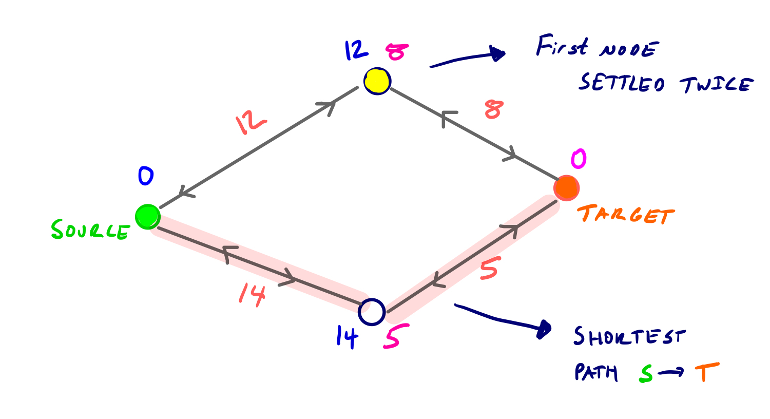
정/역 탐색 단계에서 두 PriorityQueue에서 최소값 노드를 하나씩 꺼내 처리한다고 하면 역방향 탐색에서 그림 하단 노드가 먼저 처리되고 상단의 노란색 노드가 역시 역방향 탐색에서 처리된다. 그런 다음 정방향 탐색에서 상단의 노란색 노드가 처리되는 과정으로 진행된다. 이때 동일한 노드(상단 노란색 노드)가 정/역방향 탐색에서 각각 처리되었다고 해서 탐색을 종료해버리면 실제 최단경로인 분홍색 경로는 선택되지 않는 문제가 발생한다. 따라서 실제 최단 경로는 아래와 같이 정의할 수 있다.
양방향 탐색과정에서 도달하는 모든 노드 u 에 대해, dist(s, t) = min{dist(s, u) + dist(t, u)}
이는 출발지/목적지에서 시작하는 양방향 탐색공간에 공동으로 존재하는 모든 노드들에 대해 기점으로부터 각각의 최단거리의 합이 최소가 되는 경로가 실제 최단경로가 된다는 의미이며 위 그림에서 보면 분홍색 경로가(19<20) 최단경로가 된다.
이를 좀 더 정형화 된 검증 방식으로 설명하자면 아래와 같다.
Proof of Correctness
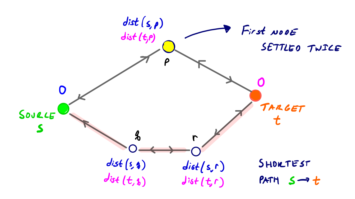
출발지 노드(s)와 목적지 노드(t), 그리고 p, q, r 노드를 갖는 위와 같은 그래프를 생각해 보자. s와 t사이 최단경로의 길이를 D라 하고 처음으로 양방향에서 각각 처리(settled)되는 노드를 p라고 할 경우 dist(s, p) = dist(t, p) = D/2 이면 p는 s와 t사이 최단경로 상에 존재하므로 탐색을 종료하면 된다.
그렇지만 위 그림은 dist(s, p)와 dist(t, p)가 D/2와 같지 않을 경우도 같이 보여준다. 이 경우는 dist(s, p), dist(t, p)가 모두 D/2보다 작을 수밖에 없는 상황이고 이는 앞서 p의 경우를 생각해보면 D/2보다 작은 최단거리를 갖는 모든 노드들은 이미 양방향에서 처리(settled)되어버렸음을 의미한다.
s와 t사이의 최단경로 상에 노드 q, r이 있고 dist(s, q) <= D/2 이고 dist(t, r) <= D/2일 경우 q는 s를 기점으로 r은 t를 기점으로 처리된 상태가 된다. 이후 링크 qr도 양 방향에서 relax된 상태이므로 q와 r노드는 결정된 최단거리를 가지게 된다.
결국 노드 s, t사이 최단경로의 길이는 dist(s, q) + dist(t, q) 와 dist(s, r) + dist(t, r)보다 작을 수 밖에 없음을 의미한다. (이 경우는 dist(s, q) + dist(t, q), dist(s, r) + dist(t, r)는 동일한 값을 가짐)
따라서, 노드가 두 번 처리(settled)된다고 해서 그 노드가 반드시 최단경로상에 있다고 보장할 수 없지만 탐색 종료 전까지 적어도 출발지(s)와 목적지(t)로부터의 거리가 결정된 노드 1개는 최단경로상에 존재하게 된다.
이제 아래의 그림을 이용해서 알고리즘의 내용을 이해해 보도록 하자.
Explanations step by step

이 그림에서 볼 수 있듯이 출발지 a에서 시작해서 목적지 e로 가는 최단경로는 [a, h, g, f ,e] 이고 이때 거리는 21이다. 이제 Bidirectional Dijkstra Algorithm을 실행하여 동일한 출발지, 목적지를 대상으로 최단경로를 찾아보자.
- 각 그래프 하단에 있는 표는 정방향 탐색(F)에서 출발지 노드로 부터의 최단거리와 역방향 탐색(B)에서 목적지 노드로 부터의 최단거리를 나타낸다.
- QF, QB는 정/역방향 탐색에서 각각 사용되는 PriorityQueue이며 이들 PriorityQueue는 [거리, 노드]로 표시되며 왼쪽 앞쪽 방향이 최단거리를 갖는 노드를 나타낸다. 예를 들어, QF의 [4, b]는 출발지 노드 a로부터 노드 b까지의 거리는 4가 됨을 나타낸다.

이제 각 단계별로 알고리즘을 이해해 보자.
- 1단계, 출발지, 목적지 노드를 정/역방향 PriorityQueue에 추가한다.
- 2단계, QB에서 최소값 노드를 poll하고(이 경우 e) Queue에 d와 f를 추가한다.
- 3단계, QF는 최단거리인 [0, a]를 가지고 있으므로 이 값을 poll하고 b와 h를 Queue에 추가한다.
- 4단계, QF가 [4, b]로 다시 최단거리를 가지므로 이 값을 poll한 다음 c를 Queue에 추가한다.
- 5단계, QF가 다시 [8, h]로 최단거리를 가지므로 이 값을 poll한 후 g와 i를 Queue에 추가한다.
- 6단계, 이제 QF와 QB가 동일한 거리 값을 가지므로 QB에서 [9, d]를 poll한다. 이제 처음으로 Join Node c를 만났으며 이때 출발지와 목적지 사이의 경로는 [a, b, c, d, e]이며 거리 μ=28이 된다. 그러나, 이는 최단경로가 되지 못한다.
- 7단계, 최단거리는 QF에 있는 [9, g]이며 이 값을poll한다. 이제 두 번째로 거리 μ=21인 Join Node f를 만난다. 이 값은 앞서 28보다 작으므로 최단경로는 [a, h, g, f, e]이며 거리는 21이 된다.
- QF.top.distance + QB.top.distance >= μ 인지 체크하며 12 + 10 >= 21이 되므로 탐색을 종료한다.
이와 같이 Bidirectional Dijkstra Algorithm을 이용하여 거리가 21인 [a, h, g, f, e]의 최단경로 탐색 과정을 살펴 보았다. 위 과정을 pseudo코드로 옮기면 아래와 같다.
while Qf is not empty and Qb is not empty:
    u = extract_min(Qf); v = extract_min(Qb)
    Sf.add(u); Sb.add(v)
    for x in adj(u):
        relax(u, x)
        if x in Sb and df[u] + w(u, x) + db[x] < mu:
            mu = df[u] + w(u, x) + db[x]
    for x in adj(v):
        relax(v, x)
        if x in Sf and db[v] + w(v, x) + df[x] < mu:
            mu = db[v] + w(v, x) + df[x]
    if df[u] + db[v] >= mu:
        break # mu is the true distance s-t
양방향의 PriorityQueue(Qf, Qb)가 공백이 될 때까지 정/역방향에서 탐색을 진행하며 frontier노드(x)가 반대편 탐색공간에 존재할 경우 출발지/목적지 사이의 경로의 거리 μ를 계산하고 이 값이 최소가 되도록 업데이트해 나간다. 즉, PriorityQueue에 포함되는 frontier노드를 이용하여 잠정적으로 만들어지는 경로의 길이가 최단거리가 되면 최단거리 경로가 되고 이때 frontier노드 x가 양방향에서의 Join Node가 된다. 위 코드 마지막 부분과 같이 출발지(s)/도착지(t) 노드로부터 정/역방향에서 처리된(settled, Sf.add(u); Sb.add(v))노드 u, v의 최단거리 합(df[u] + db[v])이 μ보다 크거나 같아지면 탐색을 종료한다. 또한 위 코드에는 표현이 되지 않았지만 최적의 결과(best result)를 도출하기 위해 정방향/역방향의 탐색공간의 크기를 서로 맞추는 것도 중요하다.
탐색 종료 후 접점노드인 Join Node를 기준으로 정방향 탐색에서 만들어진 경로와 역방향에서 만들어진 경로를 서로 연결하면 출발지와 목적지 사이의 최단경로가 만들어 진다. 이 때 주의할 점은 역방향에서 만들어진 경로는 모든 링크의 순서를 뒤집어서 연결해야 한다.
Implementation
지금까지의 내용을 Java코드로 옮기면 아래와 같은 형태가 된다. 개발자마다 구현 방법이 다를 수 있으니 참고로 생각해 주기 바란다. 코드를 보면 위에서 설명한 개념들이 어떻게 적용되었는지 대체적으로 이해를 할 수 있을 것으로 예상되어 구체적인 코드 설명은 생략하기로 한다.
/**
 * BidirectionalDijkstra.java
 */
package march.alg;

import java.time.Duration;
import java.time.Instant;
import java.util.Collection;
import java.util.HashMap;
import java.util.HashSet;
import java.util.Map;
import java.util.Optional;
import java.util.Set;

import march.graph.Graph.Dir;
import march.graph.Link;
import march.graph.Node;

/**
 * BidirectionalDijkstra algorithm implementation class.
 * The overall implementation logic came from the following article linked.
 * @see <a href="https://www.homepages.ucl.ac.uk/~ucahmto/math/2020/05/30/bidirectional-dijkstra.html">Bidirectional Dijkstra</a>
 * @see <a href="https://www.cs.princeton.edu/courses/archive/spr06/cos423/Handouts/EPP%20shortest%20path%20algorithms.pdf">Efficient Point-to-Point Shortest Path Algorithms</a>
 * @author skanto
 */
public class BidirectionalDijkstra implements Traveller {

    /**
     * Thread local variable to save Metric information of this Algorithm
     */
    private final static ThreadLocal<Metric> threadLocal = new ThreadLocal<>();

    /**
     * returns the name of this class as a algorithm name
     */
    public String name() {
        return this.getClass().getSimpleName();
    }

    /**
     * Finds an optimal path from the given source and destination node that the total cost of every node is minimal.
     * @param source a source {@link Node} object.
     * @param destination a destination {@link Node} object.
     * @return a Route object that contains information of shortest path
     * @throws IllegalArgumentException If no path is found between source and destination
     */
    public final Route traverse(Node source, Node destination) {
        final SearchSpace ss = new SearchSpace(1000);
        final MutableQueue<Node, Visit> Qf = new MutablePriorityQueue<>(700), Qb = new MutablePriorityQueue<>(700);
        final Instant start = Instant.now(); // to measure the time elapsed
        Visit vf = new Visit(source, Dir.F)/* forward */, vb = new Visit(destination, Dir.B); /* backward */
        vf.replace(null, 0, 0); vb.replace(null, 0, 0); // set initial values
        Qf.offer(vf); Qb.offer(vb);
        /* explores forward and backward direction in the order as defined, processes the same workload */
        while (!Qf.isEmpty() && !Qb.isEmpty() && !ss.satisfied(vf.cost() + vb.cost()) /* break condition */ ) {
            vf = explore(Qf, ss) /* explore forward */;
            vb = explore(Qb, ss) /* explore backward*/;
        }
        measure(start, Qf, Qb, ss); // gathers metric information
        // if mutual() is true then the two search spaces have met each other at any node in the intersection area
        if (ss.mutual()) return ss.route(); // merges each route from both search spaces
        throw new IllegalArgumentException(String.format("Path from %s to %s does not exist", source, destination));
    }

    /**
     * Do the actual processing of Dijkstra algorithm using the specified parameter information. This method can be
     * utilized to search road networks forward and backward according to the type of Queue specified as a parameter
     * @param queue PriorityQueue object it can be either forward or backward PriorityQueue
     * @param ss SearchSpace object which holds forward and backward search space information
     * @return Visit object explored
     */
    private final Visit explore(MutableQueue<Node, Visit> queue, SearchSpace ss) {
        final Visit visit = queue.poll();
        for (Node frontier: visit.frontiers()) {
            Visit adjacent = queue.pick(frontier).orElseGet(() -> visit.reach(frontier));
            if (ss.contains(adjacent)) continue; // if the adjacent node is settled already
            if (relax(visit, adjacent)) {
                if (queue.has(frontier)) queue.mutate(adjacent); else queue.offer(adjacent);
            }
            // vo - opposite Visit object
            ss.get(adjacent, adjacent.dir().flip()).ifPresent(vo -> ss.update(mu(visit, vo),  adjacent));
        }
        ss.settle(visit);
        return visit;
    }

    /**
     * Switches the cost of adjacent visit with the cost of the current visit if the cost of current visit is lower
     * than the adjacent visit as well as replaces the shortcut of adjacent with the current one.
     * @param visit the context of current visit
     * @param adjacent the context of the adjacent Node visit
     * @return {@code true} if the cost of adjacent Visit is updated otherwise returns false
     */
    protected boolean relax(Visit visit, Visit adjacent) {
        /* cost that consumes by passing through the specified link */
        final Link passage = visit.passage(adjacent);
        final float cost = visit.cost() + expense(passage); //link.elapse();
        if (adjacent.cost() <= cost) return false; /* no need to calculate hereafter */
        adjacent.replace(visit, visit.ETA() + passage.elapse(), cost); // updates previous & cost simultaneously
        return true;
    }

    /**
     * Calculates the mu(μ) value using the specified parameters. vf is a Visit object which is in the forward
     * search space and vb is a Visit object which is in the backward search space. Each vf and vb has the distance from
     * the source and destination respectively. mu is calculated as follows:
     * <ol>
     *   <li>calculate the distance from the source to the vf Visit node</li>
     *   <li>calculate the distance from the destination to the vb Visit node</li>
     *   <li>calculate the distance of link from the node of vf to the node of vb</li>
     *   <li>sums up all distances above
     * </ol>
     * @param vf a Visit object in the forward search space
     * @param vb a Visit object in the backward search space
     * @return calculated value: mu(μ) value (tentative shortest distance from the source to destination)
     */
    private final float mu(Visit vf, Visit vb) {
        return vf.cost() + expense(vf.passage(vb)) + vb.cost();
    }

    /**
     * Returns the cost of the specified link object
     * You can extend the functionality of this method if you want by applying like real time speed or road type etc.
     * @param link Link object
     * @return the cost of the specified link object
     */
    private final float expense(Link link) {
        return link.metadata.length;
    }

    /**
     * Measure the status of this algorithm. This method saves all the nodes the algorithm has visited,
     * the time it took and the count the algorithm will visit afterward in thread local variable.
     * @param start the time the algorithm starts
     * @param Qf PriorityQueue used in forward searching
     * @param Qb PriorityQueue used in backward searching
     * @param ss SearchSpae object(holds all the settled Visit objects)
     */
    @SuppressWarnings("serial")
    private void measure(Instant start, final MutableQueue<Node, Visit> Qf, final MutableQueue<Node, Visit> Qb,
            final SearchSpace ss) {
        final float elapsed = (float) Duration.between(start, Instant.now()).toMillis()/1000;
        final Set<Node> frontiers = new HashSet<Node>() {{ addAll(Qf.keys()); addAll(Qb.keys()); }};
        threadLocal.set(new Metric() { // saves metric information in the thread local variable
            public Collection<? extends Route> visited() { return ss.visited(); }
            public Collection<Node> frontiers() { return frontiers; }
            public float elapsed() { return elapsed; }
        });
    }

    @Override
    public Metric metric() {
        Metric metric = threadLocal.get();
        threadLocal.remove();
        return metric;
    }

    /**
     * This class conceptualize Search Space used in Bidirectional Dijkstra Algorithm. It holds forward search space
     * and backward search space respectively and implements convenient methods.
     * @author skanto
     */
    private class SearchSpace {
        private float mu = Float.MAX_VALUE; // the length(distance) from the source to the destination
        private final Map<Node, Visit> sf; // Forward Search Space
        private final Map<Node, Visit> sb; // Backward Search Space
        private Node node = null;

        /**
         * Constructor
         * @param initial initial search space size
         */
        SearchSpace(int initial) {
            sf = new HashMap<>(initial);
            sb = new HashMap<>(initial);
        }

        /**
         * Returns search space denoted by the direction
         * @param dir direction (Forward/Backward)
         * @return search space
         */
        private final Map<Node, Visit> space(Dir dir) {
            return Dir.F.equals(dir) ? sf : sb;
        }

        /**
         * settles the specified Visit object in the search space denoted by the direction
         * @param visit a Visit object to settle
         * @param dir direction(Forward/Backward)
         */
        void settle(Visit visit) {
            space(visit.dir()).put(visit.node(), visit);
        }

        /**
         * Checks if the specified Visit object is contained in this search space according to the direction of
         * the visit
         * @param visit visit object
         * @return return true if the specified visit is contained in this search space
         */
        boolean contains(Visit visit) {
            return contains(visit, visit.dir());
        }

        /**
         * Checks if the specified Visit object is contained in this search space denoted by the direction of
         * the visit
         * @param visit visit object
         * @param dir search direction(Forward/Backward)
         * @return returns true if a search space denoted by the direction contains the node object associated
         *  with the specified visit object otherwise returns false
         */
        boolean contains(Visit visit, Dir dir) {
            return contains(visit.node(), dir);
        }

        /**
         * Checks if the specified node object exists in the search space denoted by the direction
         * @param node a Visit node to check
         * @param dir direction(Forward/Backward)
         * @return return true if current search space contains the specified Visit object otherwise returns false
         */
        boolean contains(Node node, Dir dir) {
            return space(dir).containsKey(node);
        }

        /**
         * Finds a Visit object using the specified visit object and direction
         * @param visit a Visit object whose node acts as a key to the target Visit object
         * @param dir direction(Forward/Backward)
         * @return returns a Visit object if exists otherwise returns null
         */
        Optional<Visit> get(Visit visit, Dir dir) {
            return Optional.ofNullable(space(dir).get(visit.node()));
        }

        /**
         * Finds and returns all the Node objects search space in forward and backward holds
         * @return all the Node object as a Collection
         */
        @SuppressWarnings("serial")
        Collection<? extends Route> visited() {
            return new HashSet<Route>() {{
                addAll(space(Dir.F).values());
                addAll(space(Dir.B).values());
            }};
        }

        /**
         * checks if two(forward/backward) search spaces has met. You can suppose that a route between the
         * two search spaces is found.
         * @return returns true if the two search spaces has met otherwise returns false
         */
        boolean mutual() {
           return node != null;
        }

        /**
         * Update the existing values to the specified mu and node if the value of specified mu is less than the
         * existing value. If update is done returns true, otherwise returns false.
         * The value mu is calculated as follows:
         * <pre>
         * df[u] + w(u, x) + db[x]
         * </pre>
         * df[u] is the distance from the source to the node u in forward search and db[x] is the distance from the
         * destination to the node x in backward search. And w(u, x) is the distance(weight) from the node u to x
         * @param mu the cost(length) between the source and destination when the two search spaces is met
         * @param visit the visit object(x) which is one of visits in frontier when Dijkstra searching
         * @return returns true if specified parameters reflected on this object otherwise returns false
         */
        boolean update(float mu, Visit visit) {
            if (mu < this.mu) {
                this.mu = mu; this.node = visit.node();
            }
            return node.equals(this.node);
        }

        /**
         * check if satisfying the mu is greater than or equal to the cost and the node is settled in the forward
         * and backward search
         * @return returns true if the forward search and backward search meet
         */
        boolean satisfied(float cost) {
            return cost >= mu && node != null && contains(node, Dir.F) && contains(node, Dir.B);
        }

        /**
         * Returns Route information generated when the two search spaces meet
         * @return Route information
         */
        Route route() {
            return subroute(Dir.F).concat(subroute(Dir.B));
        }

        /**
         * Returns a Route object that has generated when the two search spaces has met
         * @param dir direction(Forward/Backward)
         * @return Route object from the search space(forward/backward) if two search space doesn't meet returns null
         */
        Route subroute(Dir dir) {
            return space(dir).get(node);
        }
    }
}
실행결과
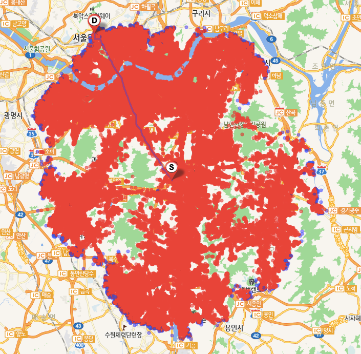
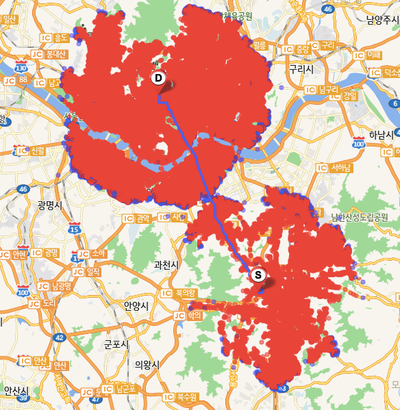
BidirectionalDijkstra Algorithm을 실행했을 때 생성되는 Search Space는 예상한 바와 같이 2개의 동심원 형태로 구성되며 서로 만나는 지점에서 출발지(판교사옥)와 목적지(광화문사옥) 사이의 최적경로가 생성된다.
또한 탐색속도는 Dijkstra: 0.5초(Node Visit: 145,888), BidirectionalDijkstra: 0.28초(Node Visit: 111,217)로 개선됨을 확인할 수 있다.
마치며…
출발지와 목적지 사이의 최단거리 찾는 알고리즘은 향후에도 여러 분야에 적용될 것이며 또한 탐색 속도 또한 중요한 경쟁력 중의 하나가 될 것이다. 오늘 소개한 Bidirectional Dijkstra Algorithm도 탐색 속도를 개선하기 위한 하나의 시도로써 기존 대비 획기적인 속도개선을 보여주는 것은 맞다. 하지만 속도를 개선함으로써 실시간성 동적 정보를 반영하는 즉, 실시간 속도정보를 반영해서 최적의 경로를 찾아주는데는 한계가 있다.
이런 문제점들에 대한 해결책으로 다양한 접근이 이루어지고 있으며 최근에는 교통공학적인 개념을 접목시킨 Contraction Hierarchy와 같은 기술들이 나오고 있다. 국내에도 이 기술을 이용하여 내비게이션 경로탐색에 접목하는 시도들이 늘어나고 있으며 구글맵과 같은 글로벌 기업들은 이미 이런 기술을 적용하고 있는 것으로 알려져 있다.
향후 기회가 되면 Contraction Hierarchy 기술에 대해 자세하게 다뤄 보고자 한다.